Jellyfish Merkle Tree in Libra Blockchain
This article introduces the Jellyfish Merkle Tree (JMT), a data structure used to store blockchain state data in Libra. The article firstly outlines the role and function of JMT in Libra and its main features; then focuses on its interface and internal implementation; finally, it compares it with Ether’s MPT tree and talks about its advantages and disadvantages.
Libra is similar to Ethernet in design, both belong to the account model, but unlike Ethernet, which stores contract data in a separate contract account, Libra abstracts contract data into Resource and stores it directly under the account (contract code Module is also stored directly into the account, code is data, both have the same status in Libra storage). The two have the same status in Libra storage). When a user uses a contract, the data generated by the contract is placed under the user’s account. The Jellyfish Merkle Tree is used to store these (account_address, resources/modules), which is important to see. But Libra uses a consensus of PBFT (with plans to move to a PoS-like consensus), and there is no such thing as a forked rollback. So the JMT implementation, somewhat different from the Ether Merkle Patricia Tree1 , does not need to consider forks.
In MPT2, the query and insertion of kv pairs start with the root_hash: H256 of a world state as the entry point of the whole tree, and the insertion of kv pairs generates a new state_root_hash, forming an incremental iterative process. With the root_hash, the upper caller can easily do a rollback operation by simply rewriting a new kv pair from one of the historical states to complete the fork.
Libra was initially designed without the concept of a block, only a transaction, or each transaction is a block in the logical sense. the version here indicates the number of transactions that have been executed on the world state, initially 0. The version represents the number of transactions that have been executed on the world state, initially 0, and the version is increased by 1 for each additional txn.
This approach is not feasible in a forkable Etherchain. Because when each forked chain forks, the state of the world after executing the same version of txn is different, otherwise it is not a forked chain.
This is one of the main features that distinguish JMT from MPT, but of course the internal implementation has also been simplified, so let’s focus on its interface and implementation.
JMT Implementation
JMT provides a relatively simple interface to the outside, a write interface, a read interface, here the main focus on the write interface (read interface is relatively simple, according to the key down addressing can be).
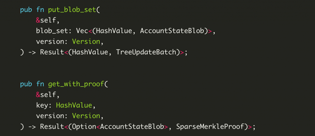
put_blob_set takes two arguments.
- One is the data to be updated, blob_set, which is essentially a list of key-value pairs, where the key is the hash of the user’s account address and the value is the serialized binary data of all resources&modules under this account, represented here by the AccountStateBlob.
- The second is the version of the transaction from which these updates are generated.
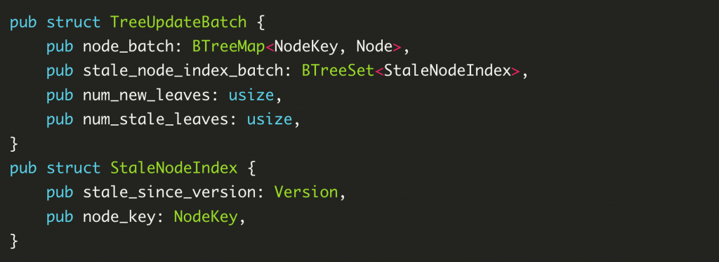
In particular, this method does not actually write the data to the underlying storage, but rather returns an update to the tree, TreeUpdateBatch, and the Merkle hash of the updated tree. treeUpdateBatch contains which nodes to add and which nodes to remove for this operation, and the caller gets this data and then caller gets this data and then performs the actual write operation.
Basic Data Structures
At this point, an introduction to the underlying data structure of JMT is needed.
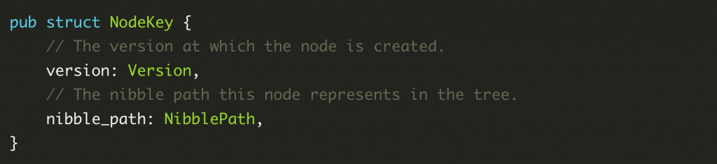
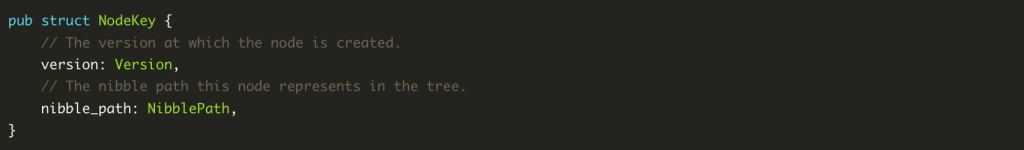
NodeKey: The NodeKey is the actual key that the underlying KV storage engine stores, and consists of two parts, version and a half-byte representation of the location in the tree, nibble_path. version of the tree.
Node: Node represents the node of the tree in JMT and is also the actual Value (serialized as binary bytes) to be stored by the underlying KV storage engine.
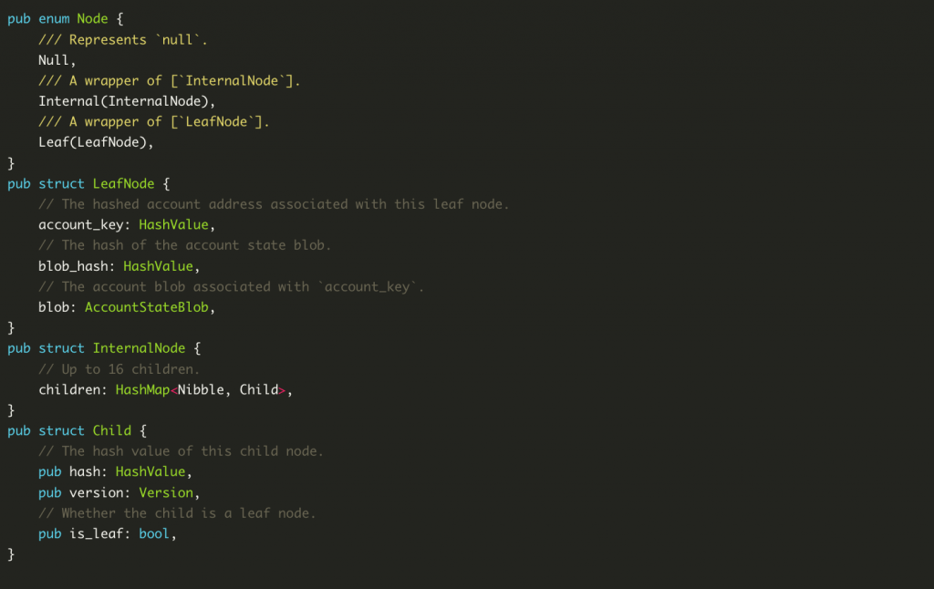
- Node::Null is the representation of the entire tree when it is empty.
- Node::Leaf Represents a leaf node of the tree. The LeadNode store’s specific account address information, as well as serialized account data.
- Node::Internaldenotes an intermediate node with children. The intermediate node is actually just a HashMap with a maximum of 16 elements, respectively, for the set of 16 nibbles, 0x00~0x0fstoring the child nodes starting with different nibbles. This is a similar design to the MPT tree.
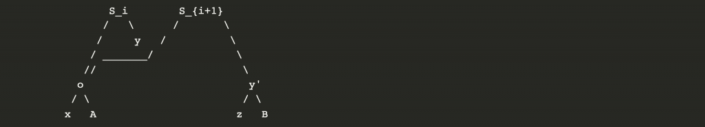
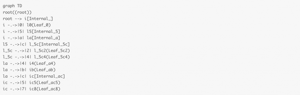
The following diagram gives a schematic representation of a possible tree structure.
The starting circular node is the NodeKey used to find the tree’s root, the solid line represents the actual physical addressing (KV mapping in the database), and the dotted line represents the logical addressing (the association in the tree). Only the physical addressing process from the root pointer to the root data is marked in the figure, and the process is omitted further down. The reader only needs to understand that for each logical addressing, there is a physical addressing process in which the parent node needs to construct the corresponding NodeKey of the child node in the store.
There are five leaf nodes in the figure.
- The address of Leaf_0 starts with0, and only it starts with0.
- The addresses of Leaf_5c2and Leaf_5c4 both start with 5c
- Leaf_a4 and Leaf_ab ground address both start with a.
- The addresses of Leaf_ac5 and Leaf_ac8 both start with ac.
The remainder of the address is omitted from the figure to avoid the address being too long and affecting the look and feel of the image.
Writing Data Flow
This section will list several common scenarios to illustrate the impact of writing data at different locations on the tree structure.
The initial state of the tree is empty.
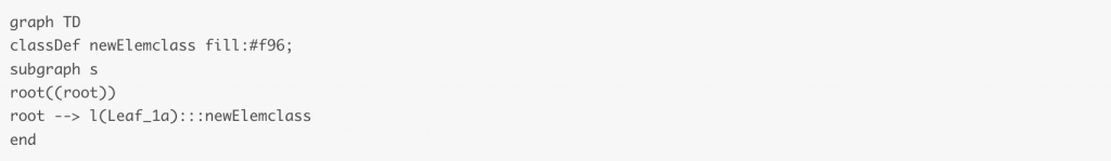
Scenario 1: Adding a node to an empty tree.
In this case, it is sufficient to construct the LeafNode directly and point the root key to it.
Scenario 2: A newly added address has the same prefix as a Leaf node.
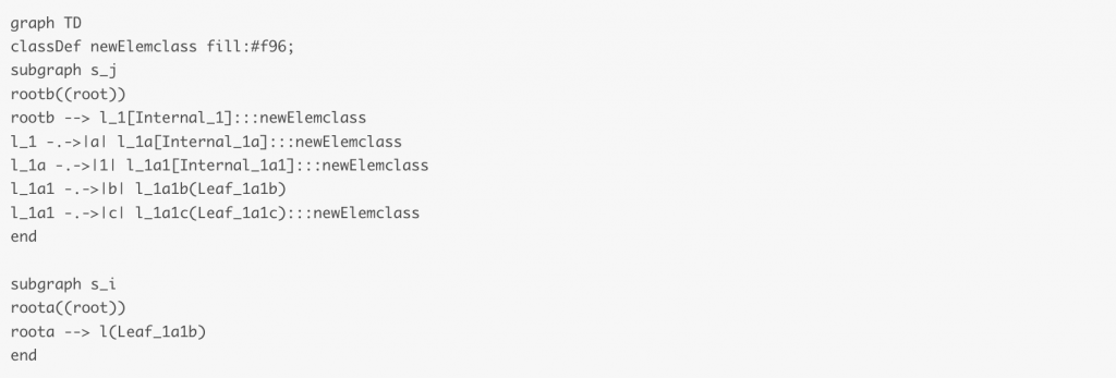
In the following figure, Leaf_1b is a newly added node, which starts with 1 as well as the existing Leaf_1a . At this point, you need to construct an Internal node and add a, b as children to your own children. (The orange color in the figure represents the new node)
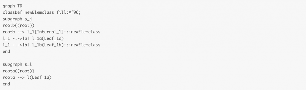
If the new address and the leaf node have more than one prefix in common, then the Internal node needs to be constructed recursively until the common parts are all Internal nodes.
Scenario 3: A new address is added that has the same prefix as the Internal node.
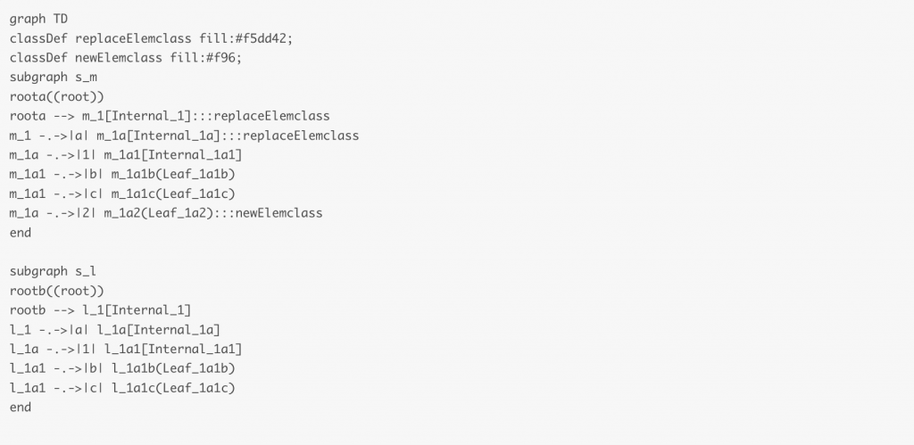
In this case, just add the new node to the children of the Internal node. In the following figure, the Leaf_1a2 node is placed in the nibble 2 slot of Internal_1a. (In the figure, the yellow node represents the node being replaced)
The three scenarios listed above cover several situations that you will encounter when writing data.
Pointer generation during physical addressing
When searching for a common prefix down the root, JMT needs to keep going to the storage engine to get the data information of the child nodes, which involves how to construct the physical address of the child nodes through InternalNode, and this section will describe this process to add this missing link.
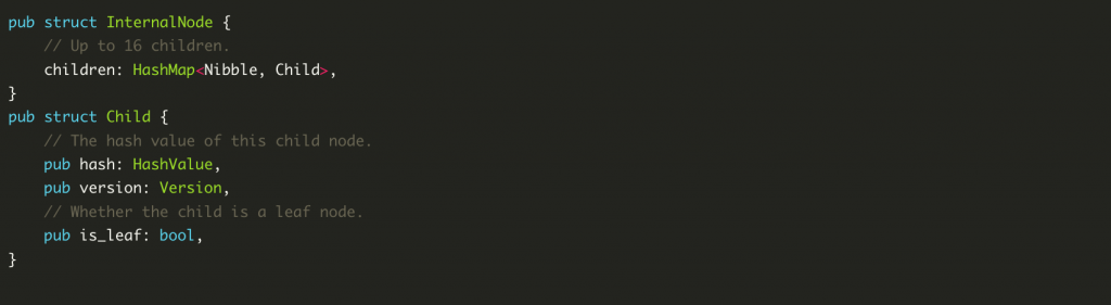
Earlier we gave the definition of the InternalNode structure, which contains up to 16 “child nodes”. The “child node” here does not store the real child data, but only a small amount of meta-information that can be used to construct a physical pointer to the child data. (Ignore child. hash, which is the hash data of child nodes cached for the purpose of calculating Merkle proof)
- child.version: the version of the child node when it was created.
- children.nibble: The “slot” where the child node is located.
- parent.nibble_path: The nibble_path of the parent node in the tree. this nibble_path is known when the parent node is addressed.
Let’s look at the definition of the physical pointer NodeKey.
With the meta-information mentioned above, you can construct the NodeKey of the child node and use this key to extract the actual data of the child node from the storage engine.
- node_key.version = child.version
- node_key.nibble_path = parent.nibble_path + child.nibble
- NodeKey of the starting root node, only version information, nibble_path is empty.
Summary
The design of JMT is actually relatively simple, except for Node::Null, there are only two typical nodes. The operation of the tree is also not complicated, and a few diagrams can basically explain it. This design is also relatively reasonable because it does not need to provide forking functionality.
But compared to MPT, JMT has a major drawback. Readers can guess what it is.
In Scenario 2, we mentioned that if the new address and the leaf node have more than one common prefix, then the Internal node needs to be constructed recursively until the common part is all Internal nodes.
What if, for example, the common prefix is too long? For example, if the first 31 bits are the same and only the last bit is different, JMT will keep constructing intermediate nodes in this case, causing the tree to become very deep.